Double Integration in Polar Coordinates

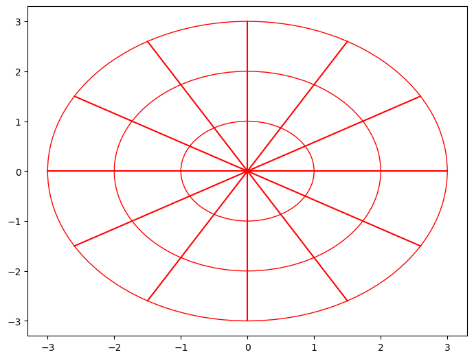
While over the past three articles, we’ve seen that double integration over cartesian coordinates is a useful and powerful tool, sometimes these integrals can be difficult to evaluate in their cartesian form. Integrating in polar coordinates by converting a cartesian double integral to its polar form or simply expressing the problem in terms of polar coordinates. Typically, integrals are defined as sums of rectangles, but this makes less sense when looking at polar regions. Let’s look at one:

# diagram of a circle with some polar rectangles
from matplotlib import pyplot, patches
import math

fig = pyplot.figure()
ax = fig.add_axes([0,0,1,1])

circle = patches.Circle((0,0), radius=3, linewidth=1, edgecolor='r', facecolor='none')
innerCircle1 = patches.Circle((0,0), radius=2, linewidth=1, edgecolor='r', facecolor='none')
innerCircle2 = patches.Circle((0,0), radius=1, linewidth=1, edgecolor='r', facecolor='none')

ax.add_patch(circle)
ax.add_patch(innerCircle1)
ax.add_patch(innerCircle2)

for angle in range(0,361,30):
    ax.plot([0,3*math.cos(math.radians(angle))],[0,3*math.sin(math.radians(angle))], color='r')

Each of the small regions in the diagram above has some of the properties of a rectangle, namely the distance from the origin of the top and bottom curves being constant, and the angle between the lines making up the sides also being constant. Given these objects are somewhat analogous to rectangles in polar coordinates, we call them polar rectangles. Let’s start by finding the area of a polar rectangle. We’re calling a portion of a circle (eg the portion from x degrees to y degrees) a wedge. Consider the following diagram of a full wedge separated into polar rectangles:

# diagram of a single wedge with contained polar rectangles marked
fig = pyplot.figure()
ax = fig.add_axes([0,0,1,1])

arc1 = patches.Arc((0,0), 6, 6, theta1=60, theta2=120, edgecolor='r')
arc2 = patches.Arc((0,0), 4, 4, theta1=60, theta2=120, edgecolor='r')
arc3 = patches.Arc((0,0), 2, 2, theta1=60, theta2=120, edgecolor='r')

for i in range(1,4,1):
    for angle in [60,120]:
        startX = (i - 1) * math.cos(math.radians(angle))
        endX = i * math.cos(math.radians(angle))
        startY = (i - 1) * math.sin(math.radians(angle))
        endY = i * math.sin(math.radians(angle))
        ax.plot([startX, endX], [startY, endY], color='r')

ax.add_patch(arc1)
ax.add_patch(arc2)
ax.add_patch(arc3)

ax.text(0, 1.5, "The polar rectangle we want", horizontalalignment="center")
ax.text(math.cos(math.radians(60)) + 0.1, math.sin(math.radians(60)), "r1")
ax.text(2 * math.cos(math.radians(60)) + 0.1, 2 * math.sin(math.radians(60)), "r2")

ax.plot(0,0)

pyplot.show()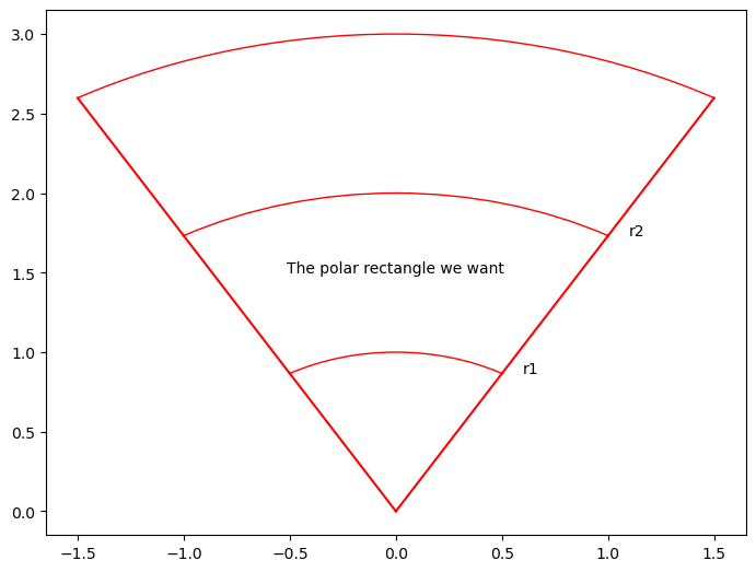

As seen in the diagram, if we take the area of the whole wedge and then subtract from that the area of the inner wedge, we will get the area of the polar rectangle that we want: $$\text{area of a wedge shaped sector}=\frac{\theta }{2\pi }\pi r^2=\frac{1}{2}\theta r^2$$ So if we take the angle between the edges to be $\theta$, the radius of the inner curve to be $r_1$, and the radius of the outer curve to be $r_2$, we get the following formulas: $$\text{area of the inner wedge}=\frac{1}{2}\theta {r_1}^2$$ $$\text{area of the outer wedge}=\frac{1}{2}\theta {r_2}^2$$ Subtracting the area of the outer edge from that of the inner wedge: $$\text{area of the polar rectangle}=\left(\frac{1}{2}\theta {r_2}^2\right)-\left(\frac{1}{2}\theta {r_1}^2\right)$$ This formula is somewhat useful, but doesn’t really lead to us our definition of the double integral for integrating over polar functions. For that, let’s introduce a couple new variables. Suppose $\mathrm{\Delta }{A}_k$ is the area of some kth polar rectangle, and then suppose $r_k$ is the average of the inner and outer radius of this polar rectangle. If we suppose that $\mathrm{\Delta }r=r_2-r_1$ (the difference of the inner and outer radii), we can say the following: $$r_1=r_k-\frac{\mathrm{\Delta }r}{2}$$ $$r_2=r_k+\frac{\mathrm{\Delta }r}{2}$$ Using $\mathrm{\Delta }\theta$ as the notion for the angle between the curves and plugging into the previous area formula, we get the following: $$\left(\frac{1}{2}\mathrm{\Delta }\theta {(r_k+\frac{\mathrm{\Delta }r}{2})}^2\right)-\left(\frac{1}{2}\mathrm{\Delta }\theta {(r_k-\frac{\mathrm{\Delta }r}{2})}^2\right)$$ $$⟹\frac{\mathrm{\Delta }\theta }{2}({(r_k+\frac{\mathrm{\Delta }r}{2})}^2-{(r_k-\frac{\mathrm{\Delta }r}{2})}^2)$$ $$⟹\frac{\mathrm{\Delta }\theta }{2}({r_k}^2+2r_k\frac{\mathrm{\Delta }r}{2}+\frac{{\mathrm{\Delta }r}^2}{4}-{r_k}^2+2r_k\frac{\mathrm{\Delta }r}{2}-\frac{{\mathrm{\Delta }r}^2}{4})$$ $$⟹\frac{\mathrm{\Delta }\theta }{2}\left(4r_k\frac{\mathrm{\Delta }r}{2}\right)$$ $$⟹\frac{\mathrm{\Delta }\theta }{2}\left(2r_k\mathrm{\Delta }r\right)$$ $$⟹\mathrm{\Delta }\theta r_k\mathrm{\Delta }r$$ Now, let’s say we want to write a partial sum to estimate the area of a polar function, $f(r_k,{\theta }_k)$, over a polar region $R$, we can do this like follows: $$S_n=\sum _{k=1}^{n}f(r_k,{\theta }_k)\mathrm{\Delta }{A}_k$$ However, when we try and turn this into an integral, we just get the following: $$S_n\approx {\iint }_{R}f(r_k,{\theta }_k)dA$$ But this isn’t very helpful since we don’t what $dA$ is. But since we know what $A_k$ is based on our work earlier, we can transform the partial sum into the following: $$S_n=\sum _{k=1}^{n}f(r_k,{\theta }_k)\mathrm{\Delta }\theta r_k\mathrm{\Delta }r$$ We can rewrite the limit of this partial sum into a useful iterated integral: $$\underset{n\to \mathrm{\infty }}{lim}{S}_n={\iint }_{R}f(r_k,{\theta }_k)rd\theta dr$$ Using a theorem from our good old friend Fubini, we can again transform this double integral into two successive single integrations: $${\iint }_{R}f(r_k,{\theta }_k)rd\theta dr={\int }_{\theta =\alpha }^{\theta =\beta }{\int }_{r=g_1(\theta )}^{r=g_2(\theta )}f(r,\theta )rdrd\theta$$

Example

Let’s try and find the volume between the XY plane and the function $f(r,\theta )=\text{something}$ in the wedge from $\theta =\pi /4$ to =$3\pi /4$ between the radii $r=1$ and $r=3$.

Double Integrals over Polar Coordinates to Calculate Area

Similar to how we can use double integrals over 2D cartesian space to calculate area, we can calulate area using double polar integrals in a similar manner. If we hold $f(r,\theta )$ within the integral constant to get rid of the volume calculation like we did for cartesian space, we get the following expression: $${\iint }_{R}rdrd\theta$$

Example

To show that this formula is consistent with all previous volume formulas, we will consider the case of the volume of a circle. We know that it is $\pi r^2$, and the integral should be equivalent. First off, we need to figure out our bounds. Since we’re going through the whole circle, our start and end angles, $\alpha$ and $\beta$ respectively, are $0$ and $2\pi$. And again since this is a circle, we can set our inner radius to be $0$, and our outer radius to be $r$, the radius of the circle. This gives us the following: $${\iint }_{R}rdrd\theta ={\int }_0^{2\pi }{\int }_0^{r}rdrd\theta$$ Evaluating the inner integral yields the following: $${\int }_0^{r}rdr=\frac{1}{2}{r}^2{|}_0^r=\frac{1}{2}{r}^2$$ Then plugging this into the outer integral: $${\int }_0^{2\pi }\frac{1}{2}{r}^{2}d\theta =\left(\frac{\theta }{2}{r}^2\right){|}_0^{2\pi }$$ $$⟹\frac{2\pi }{2}{r}^2-\frac{0}{2}{r}^3=\pi r^2$$

Transforming Cartesian Double Integrals into Polar Double Integrals

Sometimes it can be extremely difficult (or basically impossible) to evaluate an integral over cartesian space, but feasible to evaluate over polar space. This means that converting an integral from cartesian space to polar space is a useful technique. This can be done noting that $x=r\cos \theta$ and that $y=r\sin \theta$. Using these two expressions to convert an integral: $${\iint }_{R}f(x,y)dxdy={\iint }_{G}f(r\cos \theta ,r\sin \theta )rdrd\theta$$ Note also that the regions are different. $R$ is the region over cartesian space and $G$ is the region over polar space.

Example

As an example, let’s look at the following integral over the unit circle in the first and second quadrants: $${\iint }_R{e}^{x^2+y^2}dA$$ We can define the interval $R$ as being between the x-axis and the curve defined by the equation $y=\sqrt{1-x^2}$. Or more in terms of integration, we can say that the region is defined over the x-interval $[0,1]$, and the y-intervl $[0,\sqrt{1-x^2}]$. Let’s try and put this together into an integral over cartesian space: $${\iint }_R{e}^{x^2+y^2}dA={\int }_0^1{\int }_0^{\sqrt{1-x^2}}{e}^{x^2+y^2}dydx$$ Now if we even look at trying to evaluate the inner integral, we can see that it will be quite difficult, and it is in fact impossible with elementary functions. Now, let’s look at turning it into an integral over polar space: $$f(x,y)=e^{x^2+y^2}⟹f(r,\theta )=e^{(r\cos \theta {)}^2+(r\sin \theta {)}^2}$$ $$⟹e^{r^2{\cos }^2\theta +r^2{\sin }^2\theta }$$ $$⟹e^{r^2({\cos }^2\theta +r^2{\sin }^2\theta )}$$ $$⟹e^{r^2}$$ Now that we know the formula for the polar form of the function, $f(r,\theta )=e^{r^2}$, we have to find the bounds of the region in polar form. Since it’s the unit circle, we know that $0\le r\le 1$. Since we’re integrating only over the first two quadrants, we also know that we can bound $\theta$ as $0\le \theta \le \pi$. Writing this out in the form of an integral: $${\iint }_G{e}^{r^2}dA={\int }_0^{\pi }{\int }_0^1{e}^{r^2}rdrd\theta$$ Evaluating the inner integral: $${\int }_0^1{e}^{r^2}rdr$$ First, we need to do a $u$-substitution. Let’s chose $u=r^2$. Then $du=2rdr$, which implies $dr=\frac{du}{2r}$. Our bounds of integration remain unchanged since $0^2=0$ and $1^2=1$. Plugging this back into the original expression: $${\int }_0^1{e}^{r^2}rdr={\int }_0^1\frac{1}{2}{e}^{u}du=\frac{1}{2}{e}^u{|}_{u=0}^{u=1}=\frac{1}{2}{e}^1-\frac{1}{2}{e}^0=\frac{1}{2}(e-1)$$ Now plugging this into the outer integral: $${\int }_0^{\pi }\frac{1}{2}(e-1)d\theta =\frac{1}{2}\theta (e-1){|}_0^{\pi }=\frac{\pi }{2}(e-1)$$