#Using sums to find the area under the curve In the last note set I
showed you how we can use different mathematical formulas to solve
summations without figuring out every single term. I also showed you the
notation. In this note set I am going to show you how to use sums to
find the area under the curve. However, this method has some limitations
as we will see. First, lets look at some variables that will be used.
##Some variables 1. Our function in this case will be \(f\). 2. \(A_{cp}\) means the area under the curve
with our rectangles being circumcised. We will get to what this means in
a minute. 3. \(A_{ip}\) means the area
under the curve with our rectangles being inscribed. We will also get to
what this means in a minute. 4. We will be finding the area under the
curve in the set \([a,b]\). 5. \(f(u_k)\) is the minimum value of \(f\) on \([x_{k-1},x_k]\). 6. \(k\) is the index of the summation. 7. \(\Delta x\) is the width of each
rectangle/the width of each area that we are going to sum. 8. \(f(v_k)\) is the maxmimum value of \(f\) on \([x_{k-1},x_k]\) ##Rectangles We use
rectangles to approximate the area under the curve when we use
summations. If we have a graph of a function like this(we are only going
to look at the posotive areas):
 We can approximate the area under the curve by using successively
smaller rectangles. That start at the \(x\) axis, go up to the curve, and have a
width of \(\Delta x\). The sum of these
rectangles will give you the approximate area under the curve.
##Inscribed vs Circumcised Now that we know what rectangles are, lets
look at the difference between inscribed rectangles, and circumcised
rectangles. When we are creating rectangles, we need to have a height
for them. In our method currently, we are creating rectangles of width
\(\Delta x\) and a height of the
maximum value of \([x_{k-1},x_k]\) or
the minimum value of \([x_{k-1},x_k]\).
This is the difference between inscribed rectangles and circumcised
rectangles. If we are using inscribed rectangles, we are setting the
height of the rectangle to the minimum value of the function in the
interval \([x_{k-1},x_k]\). If we are
using circumcised rectangles, we are setting the height of the rectangle
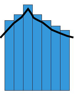
to the maximum value of the function in the interval \([x_{k-1},x_k]\). Now, lets look at some
images. A graph in which the area under the curve is being calculated
with circumcised rectangles would look like this:
We can approximate the area under the curve by using successively
smaller rectangles. That start at the \(x\) axis, go up to the curve, and have a
width of \(\Delta x\). The sum of these
rectangles will give you the approximate area under the curve.
##Inscribed vs Circumcised Now that we know what rectangles are, lets
look at the difference between inscribed rectangles, and circumcised
rectangles. When we are creating rectangles, we need to have a height
for them. In our method currently, we are creating rectangles of width
\(\Delta x\) and a height of the
maximum value of \([x_{k-1},x_k]\) or
the minimum value of \([x_{k-1},x_k]\).
This is the difference between inscribed rectangles and circumcised
rectangles. If we are using inscribed rectangles, we are setting the
height of the rectangle to the minimum value of the function in the
interval \([x_{k-1},x_k]\). If we are
using circumcised rectangles, we are setting the height of the rectangle
to the maximum value of the function in the interval \([x_{k-1},x_k]\). Now, lets look at some
images. A graph in which the area under the curve is being calculated
with circumcised rectangles would look like this:
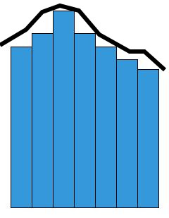
 A graph in which the area under the curve is being calculated with
inscribed rectangles would look like this:
A graph in which the area under the curve is being calculated with
inscribed rectangles would look like this:
##The summation The formula for the summation we are going to
introduce has many different limitations. These limitations are as
follows: 1. \(f\) has to continuous on
the interval \([a.b]\) 2. \((x)\) cannot be negative on any \(x\) in \([a,b]\) 3. all subintervals of \([a,b]\) must have the same length \(\Delta x\) 4. \(w_k\) has to be the minimum or maximum
value of \([x_{k-1},x_k]\) However, in
the next note set we are going to look at Riemann sums which do not have
these limitations. While Riemann sums may be more powerful, we still
need to look at using sums to find the area under the curve. Finding the
area under the curve using inscribed rectangles looks like this: \[
A_{ip} = \sum_{k=1}^{n}f(u_k)\Delta x
\] Finding the area under the curve with circumcised rectangles
looks like this \[
A_{cp} = \sum_{k=1}^{n}f(v_k)\Delta x
\] The formal defintions of these involve limits. I am going to
list them here for reference, but basically, both of them approach the
actual area \(A\) as \(\Delta x\) decreases. Here are the actual
definitions: \[
A = \lim_{\Delta x \to 0}\sum_{k=1}^{n}f(u_k)\Delta x
\] \[
A = \lim_{\Delta x \to 0}\sum_{k=1}^{n}f(v_k)\Delta x
\] This is basically saying that for every \(\epsilon\)(error rate) \(> 0\) there is a \(\delta > 0\) such that \(0 < \Delta x < \delta\). ##Conclusion
So as we have seen, we can use summations in order to calculate the area
under the curve. While the methods we were using in this note set are
not as powerful as Riemann sums or the fundamental thereom of calculus
they are still useful to know. In the next note set we are going to look
at Riemann sums and then after that we are going to look at the
fundamental thereom of calculus which allows you to find the actual area
under the curve(\(A\)) using
anti-derivatives.